26.05.2023 - Studies

Fluctuations in inflation expectations have a direct impact on stock returns and can also influence expectations regarding interest rates and the real economy. By using impulse response functions of a VAR model for the S&P 500 and its subsectors, we show that a sudden increase in inflation expectations adversely affects returns in the overall index, as well as the IT sector. Conversely, higher inflation expectations generally lead to increased returns in the energy sector. The opposite holds true for falling inflation expectations. Consumer staples are generally unresponsive to fluctuations in inflation expectations. Looking at historical prices, we find that the model's results are consistent with negative inflation shocks. We place the findings in the context of recent developments in the financial market and derive alternatives for portfolio management.
After the great financial crisis of 2007/08, the expansionary monetary policy of the central banks boosted financial markets. Low interest rates and the expansion of central bank balance sheets, however, have done little to help achieve inflation targets. For a long time, inflation remained too low from the point of view of central banks. With the unexpected return of inflation since mid-2021, central banks have had to tighten their monetary policy while trying to limit the collateral damage of higher interest rates. Since then, the financial markets have experienced major corrections. Fears of recession and uncertainty about the development of inflation increased volatility and weighed on the valuation of equity portfolios. If market participants believe that inflation has been defeated and interest rate cuts are possible again, share prices will likely rise again, as they did in the first quarter of 2023.
Overall, the centrality of macroeconomic factors on financial markets has returned to the forefront of financial market narratives due to high inflation rates and positive interest rates. This discussion is unlikely to dissipate from the agenda in the foreseeable future as a result of money overhang (Mayer, 2022) and demographic changes (Ebert, 2023).
We examine the impact of changes in the macroeconomic environment on returns in the equity market using a VAR model. Specifically, we use the model to estimate how strongly the returns of the S&P 500 and its sectors react to an exogenous shock in various macro variables such as inflation and short-term interest rates. Finally, we investigate the extent to which the relationships of the VAR model are reflected in historical price developments and simulate portfolios with different macro sensitivities.
The key takeaway is that equity returns are particularly responsive to shocks to inflation expectations. The overall index has reacted negatively to rising inflation expectations, primarily due to the strong negative reaction of the IT sector. Conversely, the energy sector has reacted positively, but its gains cannot fully offset the negative effects of the IT sector. Consumer staples proved to be relatively insensitive to inflation shocks. The developments in share prices over the past two years further confirm this trend. A cut in interest rates would likely trigger a short-term rally in the IT and real estate sectors. However, this effect would be short-lived as it would fuel inflation and subsequently place downward pressure on yields once again.
While older research papers often used actual macroeconomic variables such as GDP growth or consumer price index growth (see, for example, Ang et al., 2012), our approach relies on market expectations, as described by Esakia and Goltz (2022). The reason is that market players are forward-looking, and market prices are based on available information and associated narratives (Kleinheyer and Mayer, 2020). We rely on fixed-income securities prices to derive expectations for the development of macroeconomic variables, using breakeven inflation, which is the difference between the yield of inflation-linked and nominal government bonds, as a measure of inflation expectations. Our analysis focuses on the U.S. market due to its high liquidity and availability of data. The financial market variables that reflect our expectations about the macroeconomic environment are as follows:
Table 1 shows the basic properties of the macro variables. The statistics of the first row are based on the monthly return of the S&P 500:

with t in months. The abbreviation TR stands for Total Return, i.e. price changes of the S&P 500 including dividends. The average monthly return of the S&P 500 between January 1962 and April 2023 was 0.89%, i.e. approximately 11% annualized. The fluctuations are large: from September to October 1974 there was the highest monthly return of 16.78% and between September and October 1987 the lowest with minus 21.54%.
The macro variables are available for different time periods and fluctuate at smaller scales. For instance, the 10-year breakeven inflation (BEI10Y) has ranged between 0.24% in December 2008 and 3.27% in April 1997, and the short-term interest rate (3M Treasury) has ranged between 0.01% in December 2011 and 15.6% in September 1981.
Results of various linear regressions confirm our choice of a VAR model for analysis. First, multivariate regressions that extend the bivariate regressions of Esakia and Goltz (2022) show that the results of this approach are biased, especially because it does not consider the endogenous interaction of the variables. Second, regressions over rolling time windows show that the relationship between the variables is not constant over time and that the history of the variables plays a relevant role (see Online Appendix A1). We can explicitly model both with a vector autoregression (VAR) model.
With a VAR model, all variables are modeled as potentially interdependent.1 Each variable is explained by its own past as well as the history of the other variables. The interaction of all variables is thus explicitly modeled. In our case, this means that macro variables and index returns influence each other over time as part of a system. Specifically, we use breakeven inflation2 and the term spread as indicators of expectations about inflation and the business cycle. We also include in the model the three-month U.S. Treasury yields as an indicator of short-term interest rates and the credit spread as an expression of the market's risk premiums for bad credit ratings.3
Our VAR model is a system with five equations, where the rate of return and each macro variable are each on the left-hand side, while their own past, as well as the past values of all the other variables are on the right hand side of each equation. We estimate the model in levels based on monthly data. We use a total of 12 lags, i.e. the history of the last year and thus take into account more than just the immediate past.
First of all, the results confirm that the model has been specified correctly: all variables influence each other. A Granger causality test, which examines the contribution of the past of the other variables and their past to the explanation of each variable in the system, confirms the importance of the macro variables and their interactions. In particular, in the equation in which the return is isolated to the forecast on the left side, all macro variables on the right side of the equation make a significant explanatory contribution (see Appendix A2).
The VAR model can be used to model hypothetical exogenous shocks and observe their consequences through the impulse response function. This function tracks the effects of a one-standard deviation exogenous change to a single macro variable on the overall system while holding other variables constant. This enables us to monitor changes in returns over time caused by an isolated shock to a single macro variable. The impulse response function shows the influence of a shock as a deviation from the mean return each month after the shock. In turn, we can obtain the cumulative impulse response function CIRFt by summing up these influences each month up to t.
Therefore, CIRF0 gives the immediate return effect, CIRF1 the total effect after one period, CIRF2after two periods and so on. Figure 1 shows the cumulative impulse response function for the S&P 500 return after shocks of the four different macro variables. Since the impulse response is symmetrical by design, it is sufficient to investigate positive shocks. In the case of negative shocks, only the sign of the results is reversed.4
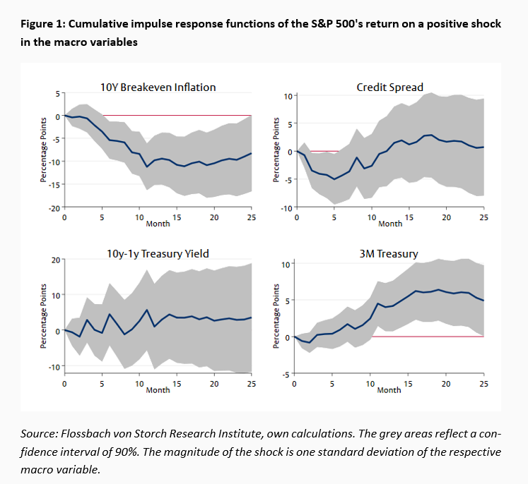
The blue line represents the month CIRFt after month t from the time of the shock. The grey area marks the confidence interval for a probability of error of ten percent, i.e., the probability that the blue line is actually outside the grey area is ten percent.
According to the model, a positive exogenous shock in the change in breakeven inflation by one standard deviation, which corresponds to 44 basis points, does not initially lead to a significant change in yields. After five months, however, the cumulated returns are almost four percentage points lower than in the absence of a positive shock, although the effect is not yet statistically significant. After 15 months, yields are almost 11.5 percentage points lower than before the shock. It is always assumed that nothing else has changed structurally in the model and that no further shocks have occurred.
An unexpected widening of the credit spread of 43 basis points, or an empirical standard deviation, provides a cumulative negative effect on yields of 7.8 percentage points over six months. However, this effect disappears quickly. A shock from the yield curve has no clear effect on yields over time. A positive impulse from the short-term interest rate of 32 basis points (one standard deviation) initially leads to a slight cumulative decline in monthly returns of almost 90 basis points, but after 15 months it leads to a cumulative positive effect of more than 5 percentage points. Yields are the most responsive to changes in inflation and interest rates.
An example helps illustrate the impact of the breakeven inflation shock: the monthly return of the S&P 500 between the beginning of 2009 and the end of 2019 averaged 1.22%. If the S&P 500 continued to rise in the same trend, the cumulative monthly return would be 6.1% five months later (1.22% times five months). Assuming there is a positive shock from breakeven inflation of 44 basis points (one standard deviation), the cumulative effect on the yield after five months would be minus four percentage points according to the impulse response (see Figure 1, upper left chart). The added return after five months would therefore be a total of 2.1% (6.1% average return minus 4% due to the inflation shock). After 15 months, the cumulative monthly return without shock would be 18.3% and the cumulative effect of the shock would be minus 11.5 percentage points. The cumulative return after 15 months of shock would therefore be only 6.8%. Figure 2 shows these effects converted into the associated price changes of the S&P 500 using the example of a shock in January 2020. We normalized the price to 100 at the time of the shock.
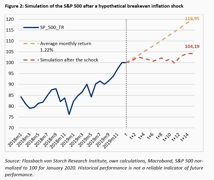
Assuming monthly growth of 1.22%, the S&P 500 would be 19.95% higher after 15 months due to compound interest. However, if there is a one standard deviation breakeven inflation shock, the S&P 500 will only be 4.19% higher after 15 months because of the effect on the monthly returns.
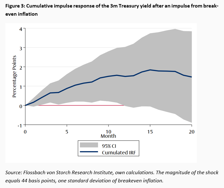
Since the VAR model represents a system in which all variables depend on each other, we can also take a closer look at the impact of a change in inflation expectations on short-term interest rates. If inflation expectations change, central banks also react and, as a result, short-term interest rates. The variables influence each other. Figure 3 shows the effect of a breakeven inflation shock on short-term interest rates, i.e. the 3-month US Treasury yield. The short-term interest rate reacts quickly to an inflationary shock and shows a significant correlation in the first 10 months. After that, the cumulative effects are no longer significant.
The responses of yields to breakeven inflation and short-term interest rates movements, as well as the reaction of interest rates to inflation, fit a pattern that we have observed since mid-2021, albeit with a slightly longer time lag: After an inflationary jump, the stock market remained optimistic for a brief period with the view that inflation was transitory and rate hikes were not needed. However, when inflation did not subside, central banks were compelled to raise interest rates. Price losses came with disillusionment.
We now look at sectoral differences and focus first on the breakeven inflation because it showed statistically and economically significant results at the index level. Also the Fed's interest rate hikes since March 2022 have been responses to rising inflation. The cumulative impulse responses of the returns of the individual sectors of the S&P 500 show significant differences (Figure 4).
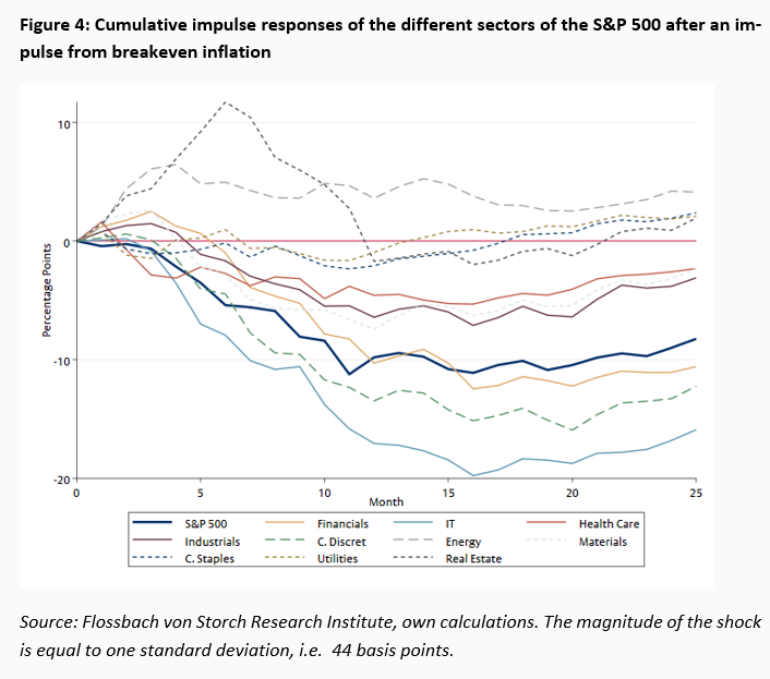
The very positive short-term development of the real estate sector of more than 10% cumulative effect is striking. After just over a year, however, it is already completely consumed again. In the first six months after an inflation shock, the real estate sector can thus act as a hedge against inflation. However, as soon as inflation-induced interest rate hikes occur, the pressure on real estate valuations and loans reduces yields again.
In absolute terms, the IT industry is the most responsive to changes in inflation expectations. An increase in inflation expectations of 44 basis points (one standard deviation) results in a cumulative effect of minus 7 percentage points after five months. After 15 months, the effect adds up to minus 17.6 percentage points. If the index of the technology sector were to rise by 1.66% per month, as it did on average between 2009 and 2019, the accumulated monthly return would be 24.9%. With the shock, this cumulative yield decreases by 17.6 percentage points to 7.3%.
Figure 5, analogous to Figure 2, shows the impact on the simulated price movements of different sectors of the S&P 500 due to a shock in the breakeven inflation.
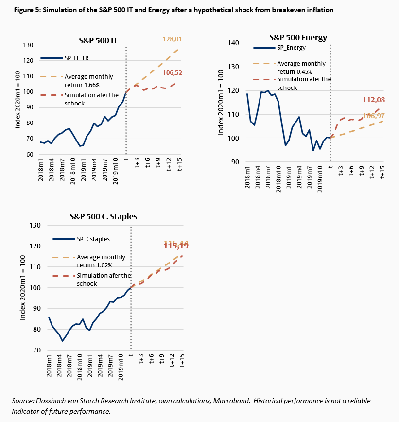
Over 15 months, the IT sector is performing more than 21 percentage points worse than without a shock. At the other end of the spectrum is the energy industry. In our model, a shock in inflation expectations of 44 basis points leads to a cumulative effect on yields of around six percentage points after just 4 months. Fifteen months after the shock, the index would be 12.08% higher, but only 6.97% without the shock. The consumer staples sub-index remains largely unaffected.
The results, as at the index level above, are consistent with recent experience since the last sharp change in inflation expectations in the summer of 2021. Changes in energy demand take time and are, if at all, only possible to a limited extent. Relative to all other sectors, price increases can therefore best be passed on. In the IT sector, the picture was mixed. First reference was made to the pricing power of the market leaders in particular and inflation was considered unproblematic. After some time, however, the focus was on interest rate hikes following the rise in inflation. Due to the associated depreciation of future cash flows, IT stocks lost value. Consumer staples proved to be inflation resistant. The associated narrative was: In times of high inflation, it is possible to switch to cheaper products in the short term. However, food is always needed.
Over the past two years, central bank interest rate hikes have been driven by inflation expectations. In the wake of the bankruptcy of American regional banks, there was a growing suspicion that central banks could unexpectedly cut interest rates out of concern for financial stability, regardless of inflationary developments.
This change would be exogenous to the VAR system modeled here and its influence can also be estimated using impulse response functions. The impulse response function of yield and breakeven inflation to a negative shock of the short-term interest rate is shown in Figure 6.
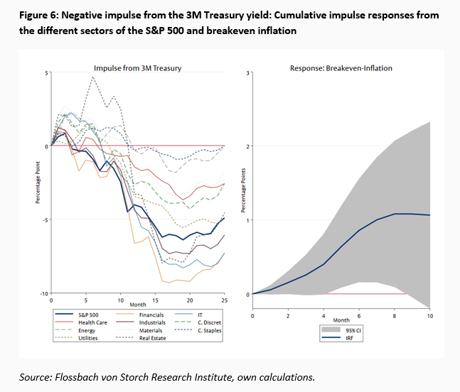
An exogenous cut in the short-term interest rate by 32 basis points (one standard deviation) would have a positive effect on energy sector retruns of almost two percentage points after just two months. However, this would disappear within a year. Yields in the IT sector initially rise at the same rate as those in the energy sector but fall sharply from the eighth month onwards. Consumer staples are barely reacting to the interest rate shock. According to our VAR model, the real estate sector would be the biggest beneficiary six months after an exogenous rate cut. After ten months, however, the cumulative effect would also be negative. The reason is that a rate cut will – in the medium term - fuel inflation. A short-term relief of the financial market would have been bought index-wide with long-term pressure on valuations.
We now investigate the extent to which the correlations from the VAR model can be historically proven. Due to the assumptions that the shock occurs in isolation in the model and that the system otherwise does not change structurally, and because we cannot clearly identify pure exogenous shocks in real prices, quantitative deviations occur in this historical review. In terms of quality, however, the results from the VAR model are largely valid.
Basically, from the VAR model analysis, we expect the returns of the entire S&P 500 to be lower after an exceptionally strong positive move in breakeven inflation changes than they would have been without such a shock. What would be needed is for the movement in breakeven inflation to be "exogenous" and not just a reaction to movements of other variables. In addition, because the VAR model assumes symmetry in the response to the shocks. We would expect that an equal decline in the change in breakeven inflation, i.e. a negative shock, would lead to higher returns in subsequent periods. For the IT sector, we expect analogous behavior. In the energy sector, the opposite relationship should be seen.
We measure the levels of inflation expectations and yields. Thus, the individual historical shocks that we examine below have a greater time gap from each other than when viewed monthly. Thus, the results are more compatible with the impulse response analysis, which assumes isolated shocks. Figure 7 gives a first glimpse of how S&P500 returns move after changes in breakeven inflation.
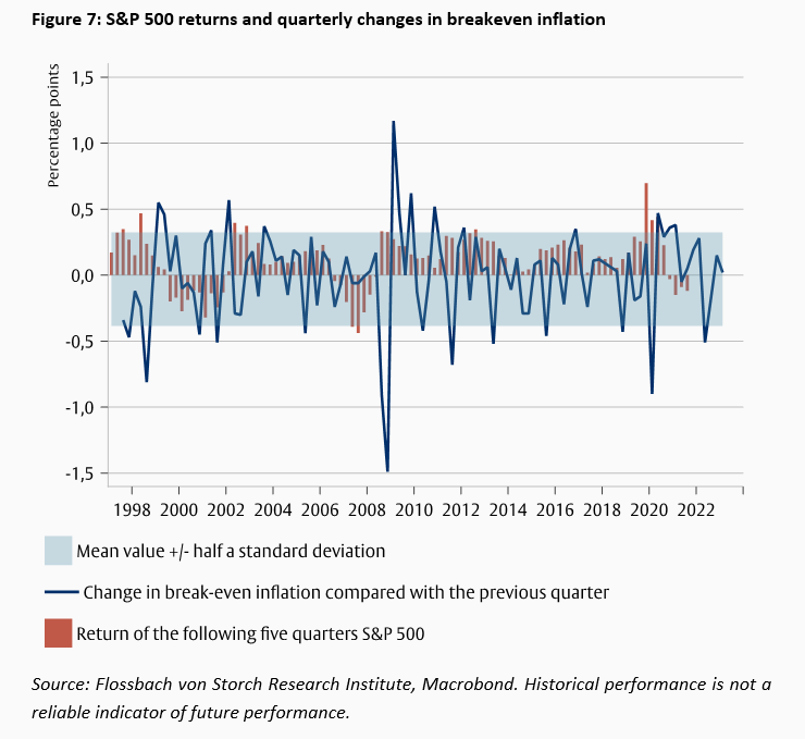
We focus on extraordinarily large changes in breakeven inflation, which we call an "empirical inflation shock." An empirical inflation shock occurs when the absolute change in breakeven inflation, represented by the blue line, exceeds the absolute quarterly average change calculated over the entire observation period by more than half a standard deviation in a quarter. This represents a change of more than 32 basis points. Quarters with an "inflation shock" can be identified in Figure 7 by the fact that in such quarters the blue line leaves the light blue shaded area. As a "reaction", we look at the return of the S&P 500 in the 5 quarters after an empirical inflation shock. Figure 7 shows the total return for the next five quarters following a quarter with red bars.
The negative shocks occur approximately every two years between 1997 and 2001 and 2008 and 2020. The positive shocks are concentrated in the period around the turn of the millennium, in the years 2009 and 2010 as well as in the recent past since 2020. We can't pinpoint exactly which changes are exogenous. However, the very large changes between 2008 and 2010 do not seem exogenous to us, but a reaction to the upheavals of the financial crisis. The shocks during this period came from the financial sector, not from a change in inflation expectations. That is why we leave this period out of the investigation.
In the 62 quarters considered since 1997, we find a total of 20 quarters with an empirical inflation shock. Eight of them are positive and twelve are negative. The average absolute empirical shock is 49.5 basis points, which is almost identical to the 44 basis points, or one standard deviation used in the impulse response function above, making the results comparable. Between 2011 and 2020, there seems to be a tendency to see a synchronization between deflationary shocks and above average positive returns.
Looking at the IT and energy sectors, two sectors with prominent impulse responses in the VAR model, suggest patterns: In the IT industry, positive shocks are increasingly occurring with low or even negative future returns. Negative shocks seem to result in higher returns than the average. In the energy sector, it is the other way around (Figure 8).
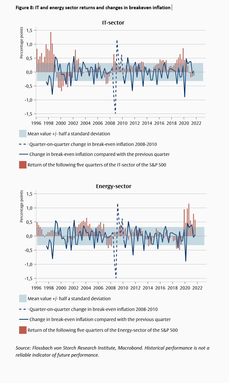
The visual impressions can be confirmed statistically. Table 2 shows the averages of rolling 5-quarter returns overall, as well as broken down by positive and negative inflation expectation shocks for the index as a whole and for selected sectors. The numbers thus correspond to the red bars from Figures 7 and 8.
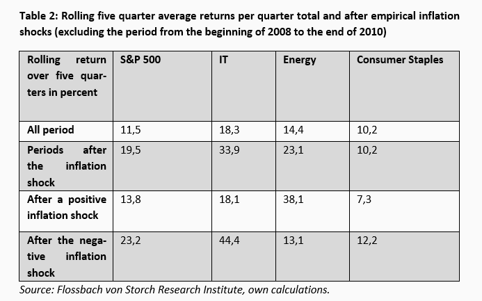
If one distinguishes between positive and negative shocks (penultimate and last line of Table 2) in the individual sectors compared to the yield level of all periods (first row), one finds some of the correlations from the VAR model. The model predicts that the returns of the overall index would move in the opposite direction of the shock. Historically, this applies to negative shocks, but not to positive ones. After a negative inflation shock, the returns of the overall index are significantly higher than the average for all periods. After positive shocks, however, yields are also, albeit slightly, above the return for all periods.
By sector, the asymmetric development of yields after shocks can also be seen. On the average historical inflation shock, the IT sector sees an average deviation of minus 0.2 percentage points compared to the average of all periods with positive inflation after 5 quarters. In the event of a negative shock, the average return is 26.1 percentage points higher than in all periods. Yields in the energy sector are only 1.3 percentage points below average in the event of a negative shock. In the case of a positive shock, however, they are 23.7 percentage points higher. Thus, this simple historical review confirms the different directions of inflation in these two sectors as predicted by the VAR model. However, the magnitude of the impact varies depending on the direction of the shock.
Consumer staples react almost symmetrically to positive and negative inflation shocks and also have the same qualitative deviation as predicted in the impulse response of the VAR model. There is only a 4.9 percentage point difference in yields between positive and negative shocks. The average return for the periods after inflationary shocks is identical to that of all periods.
Tracking the historical performance of the S&P 500 and inflation expectations since 2018, our analysis provides practical implications for portfolio management. Figure 9 shows the price performance of the complete S&P 500 as well as excluding the energy and IT sectors (all normalized to 100 as of January 1, 2018). Inflation expectations as measured by breakeven inflation are shown in the lower panel.
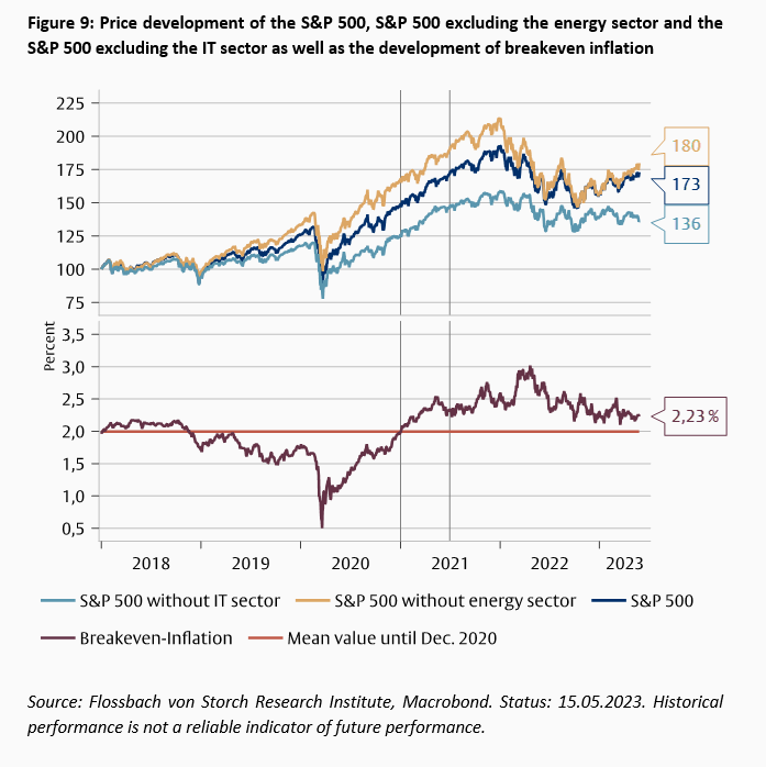
The remarkable impact of technology stocks on the overall index is evident. Had investors divested from the IT sector, they would have suffered a 30-percentage point loss in returns from the beginning of 2018 to May 2023 compared to the overall index. The higher yields are primarily due to the period up to the end of 2020, when inflation expectations remained below their historical average of 2% and the US Federal Reserve implemented an aggressive monetary expansion in response to deflationary fears after the pandemic shock in Spring 2020. The 23-percentage point spread between the index with and without the IT sector by the end of 2020 highlights how the IT sector benefited from periods of low inflation expectations and greater liquidity to underpin the overall index.
The energy sector presents a different story, with its contribution to the overall index being slightly negative. Since 2018, the index excluding the energy sector has outperformed the overall index by six percentage points as of May 2023. Notably, during periods of low inflation expectations and exceptionally high liquidity until the end of 2020, the energy sector's hindering impact on yields is conspicuous.
In the first half of 2021, CPI inflation rates exceeded the US Federal Reserve's 2% inflation target, and breakeven inflation also crossed the 2% threshold for the first time in two years. Although the common belief at the time was that inflation was transitory, the large-scale expansion of central bank balance sheets and the expansionary fiscal policies during the pandemic casted doubt on whether the trend would be temporary (Mayer 2020). The continuously increasing inflation expectations throughout mid-2022 further supported this view. As a result, the US Federal Reserve reacted to inflationary pressures with multiple interest rate hikes from March 2022 onward. If an investor had chosen to invest in the S&P 500 from mid-2021 until the end of 2022 while excluding the energy sector despite rising inflation expectations, she would have incurred an 8.4 percentage point loss compared to an investment in the overall index.
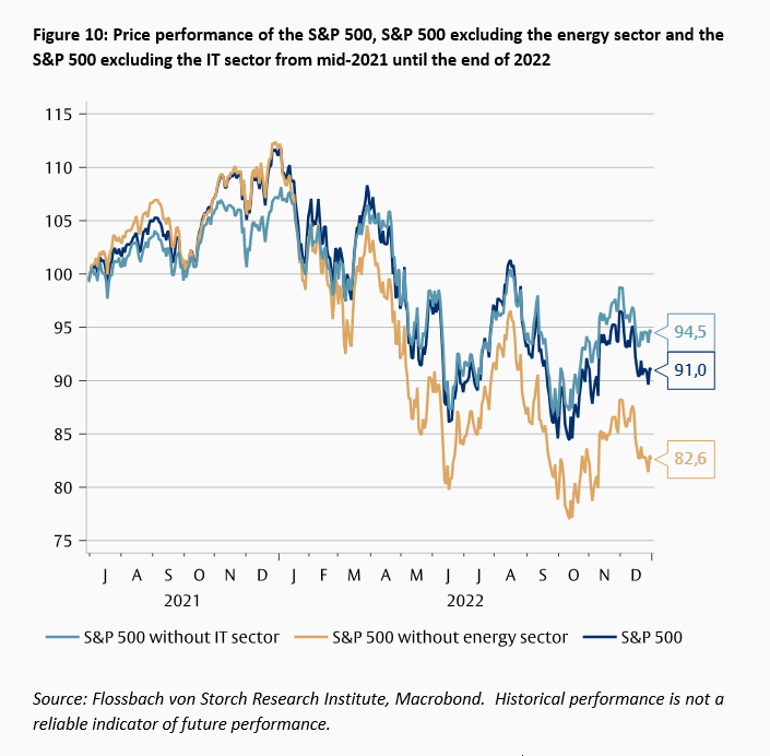
Despite having a sector weight of less than 5%, the energy sector has significantly contributed to the overall index during the past 18 months. In comparison, excluding the IT sector, which tends to be inflation-prone, would have resulted in an additional 3.5 percentage points of returns. Although the IT sector has a sector weight of around 25%, its influence is moderate. Nonetheless, our historical findings and the VAR model confirm that when inflation expectations decline, the energy sector has a negative reaction, while the IT sector reacts positively. Conversely, when inflation expectations rise, the opposite trend occurs.
As the new year began, an increasing number of market participants believed that the battle against inflation had been won, resulting in a decrease in inflation expectations and the solidification of expectations for monetary policy expansion. Since January 2023, there has been a reversal in sectoral performance, as shown in Figure 11.
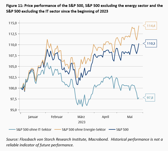
The upswing in the overall index is largely due to the rally in IT stocks, while the momentum of energy stocks has slowed down. This trend is reminiscent of the period between the start of 2018 and the end of 2020, when low inflation expectations and the consequent monetary policy relaxation were beneficial for the technology sector. As a result, technology stocks experienced a boost, while the attractiveness of energy stocks waned.
The dominant narrative of defeated inflation in the market may soon face challenges, and only time will tell how long it will remain relevant. One potential scenario is that central banks may cut key interest rates due to fears of a financial crisis, resulting in a shock to the market that differs from inflation expectations. According to our VAR model, such a surprising rate cut would lead to a short-term recovery in the IT and energy sectors (Figure 6), but could lead to a resurgence of inflation in the long run. While the trigger may differ, the resulting story will likely resemble the period from summer 2021 to the end of 2022, leaving financial investors with similar options as in that time frame.
The prolonged period of low interest rates, high liquidity, and deflationary fears, prevalent for over a decade, has now come to an end with the onset of high inflation rates in recent times. To assess the impact of changes in the macroeconomic scenario on equity returns, we used the S&P 500 and analyzed the changes in market expectations derived from fixed income prices. Our analysis indicates that changes in inflation expectations have the greatest impact on shaping the economic environment as they influence interest rate and business cycle projections.
Impulse response functions of a VAR model show that a positive exogenous shock of 44 basis points (one standard deviation) in inflation expectations, as measured by breakeven inflation, initially has little effect on the monthly returns of the S&P 500. However, compared to the pre-shock baseline, the effect on yields adds up to almost four percentage points after five months and 11.5 percentage points after 15 months. For example, if the monthly return before the shock was 1.22% (as on average between 2010 and 2019), it would add up to 6.1% after five months without shock. A positive inflation shock would reduce this by 4 percentage points to 2.1%. Normalizing the index to 100 at the time of the shock, the price of the index would have risen to only 104.19 points 15 months after the shock. Without shock, it would stand at 119.95. According to the VAR model, the shock therefore causes performance to be reduced by around 15 percentage points five quarters after a positive shock in inflation expectations.
The effects differ for the different industries. The IT sector reacts most strongly to a positive shock of breakeven inflation with a fall in yields. The effect on the energy sector is reversed. The positive shock in breakeven inflation leads to a cumulative effect on monthly returns of plus 6 percentage points within 4 months. This effect persists after 15 months. Returns on the consumer staples index remain broadly unchanged.
An interest rate cut that is not driven by deflationary expectations, but e.g. triggered by concerns about financial stability would have a short-lived positive effect on yields. The IT sector would benefit most from this and, belatedly, the real estate sector. However, because an interest rate cut fuels inflation again, the cumulative effect would be negative overall after 15 months.
Our findings suggest that investors can minimize macroeconomic risks in equity portfolios by diversifying appropriately. To protect against a decline in inflation expectations, adding shares from the IT sector would be a suitable strategy. Conversely, benefiting from positive changes in inflation expectations could be achieved by investing in the energy sector. Consumer staples, however, are minimally impacted by macro risks. These insights can guide investors in building a diversified portfolio that is positioned to weather macroeconomic changes effectively.
Ang, A., Brière, M., & Signori, O. (2012): Inflation and individual equities. Financial Analysts Journal, 68(4), 36-55
Ebert, Sven (2023): "Demography and Interest Rate Turnaround", Commentary, Flossbach von Storch Research Institute.
Enders, W. (2008): Applied econometric time series. John Wiley & Sons.
Esakia, M., & Goltz, F. (2022): Targeting Macroeconomic Exposures in Equity Portfolios: A Firm-Level Measurement Approach for Out-of-Sample Robustness. Financial Analysts Journal, 1-21.
Kleinheyer, M., & Mayer, T. (2020): Discovering markets. Quarterly Journal of Austrian Economics, 23(1), 3-32.
Lütkepohl, H. (2013): Introduction to multiple time series analysis. Springer Science & Business Media.
Mayer, Thomas (2020): The Inflation Puzzle, Commentary of 09.06.2020, Flossbach von Storch Research Institute.
Mayer, Thomas (2022): The "monetary phenomenon", Study, Flossbach von Storch Research Institute.
1 For an introduction, see, for example, Lütkepohl (2013).
2 Breakeven inflation and 5y5y forward rates differ little from each other in their characteristics, but breakeven inflation is available for a longer period of time. Therefore, for further analysis, we only use breakeven inflation to measure inflation expectations.
3 All macro variables except for the returns of the 3M Treasury are stationary in levels. For 3M treasury, we take the differences to ensure stationarity.
4 See Enders (2008, p. 273f) for the formal definition of an impulse response function and how it is derived from the VAR model.


